Project 6 - Monte Carlo Computation of Pi using MIPS Floating Point

Goals

In this project you will work with programming MIPS to use floating point data and instructions to compute pi.

Floating Point in MIPS

As we have seen, there are different representations for integer and real numbers. We have seen several ways of manipulating integers and this project will focus on floating point values.

Like most computer systems today, MIPS uses the IEEE-754 standard to represent both single precision (32 bit) and double precision (64 bit) floating-point representations. The MIPS intructions are described in Appendix B (starting on page B-73). Floating-point operations are performed on a floating-point coprocessor that contains 32 general purpose floating point registers, $f0 through $f31 (click the Coproc 1 tab in MARS to see these registers). Each register holds only 32 bits, only enough for a single precision value. Double precision values are stored in two adjacent registers, and are referred using the smallest register number. For example, a double precision value stored in $f0 and $f1 would be referred to as $f0.

Imagine you would like to convert a temperature in degrees Celsius to degrees Fahrenheit. The program float.s shown below illustrates one way to do this. Download and run this program, stepping through the program and watch the memory and the register values change.

# Temperature Conversion C -> F

.text

main:

# Get the temp in C from user
	li	$v0, 4		# Load 4=print_string into $v0
	la	$a0, prompt	# Load address of prompt into $a0
	syscall			# Output the prompt
	li	$v0, 6		# Load 6=read_float into $v0
	syscall			# $f0 contains float


# Conversion from C to F: F = 32 + C*180/100

	l.s	$f1, c1		# conversion factor 1
	l.s	$f2, c2		# conversion factor 2
	mul.s	$f3, $f0, $f2	# C*180/100
	add.s	$f3, $f3, $f1	# F = 32 + C*180/100
	mov.s	$f12, $f3	# Copy $f3 to $f12
	li	$v0, 2		# Load 2=print_float into $v0
	syscall			# print value in $f12

	li	$v0, 4		# Load 4=print_string into $v0
	la	$a0, newline	# Load address of newline into $a0
	syscall			# Output the newline


# See if it cold
	l.s	$f1, c3		# $f1 = constant 0.0
	c.lt.s	$f3, $f1	# compare temp and 0
	bc1f	endif		# brach if temp is negative
	li	$v0, 4		# Load 4=print_string into $v0
	la	$a0, cold	# Load address of string into $a0
	syscall			# Output the string
endif: 


# Exit Gracefully

	li	$v0, 10
	syscall


.data
	.align 0
n:
	.word 10
c1:	.float 32	# conversion factor 1
c2:	.float 1.8	# conversion factor 2
c3:	.float 0.0	# cutoff for "cold" temperature
prompt:
	.asciiz "Enter the temperature in Celsius: "
cold:
	.asciiz "Brr.  That is C-O-L-D!!!\n"
newline:
	.asciiz "\n"

Here are some important things to note about the above program. There are floating point instructions for single precision and double precision, specified using either .s or .d respectively. Note the .float directive in the .data section can be used to store floating point values in memory that can be loaded into a floating point register using the l.s instruction. There are no immediate type floating point instructions (can you imagine why not?). A wide variety of comparisons are available (similar to beq, bne, etc) that set a flag in the floating point coprocessor. One of these is the c.lt.s instruction, which sets the flag if the first operand is less than the second operand. The flag can be checked using the bclf instruction, which branches if the flag is false; bclt branches if the flag true. Also, note there are specific system calls for reading and printing floating point values.

Pseudo-Random Numbers

Most computer languages provide a mechanism for producing random numbers called a random number generator (RNG). These random number generators produce numbers that are deterministically computed therefore are not truly random. In fact there are no truly random numbers available on a computer, because computers always produce the same results for a given set of inputs. A complete discussion of how computers compute pseudo-random numbers is beyond this project, but see the Knuth reference or talk to me if you are interested in learning more.

Pseudo-Random Numbers in MARS-MIPS

The MARS simulator has available a few system calls related to random numbers (these are not available in SPIM). Of particular importance in our application here is setting the initial seed value, setting the range of random numbers, and obtaining random numbers. The program random.s shown below illustrates how to compute random numbers in MIPS using MARS.

.text main: # Initialize the random number generator seed li $a0, 0 # Load RNG ID (0 in this case) into $a0 li $a1, 314 # Load RNG seed (314 in this case) into $a0 li $v0, 40 # Load 40=set_seed into $v0 syscall # Initialize RNG via syscall # Compute and print n random floating point values la $t4, n # address of n lw $t4, 0($t4) # t4 = n and $t0, $0, $0 # i = 0 loop1: # Compute Random Number li $a0, 0 # Load RNG ID (0 in this case) into $a0 li $v0, 43 # Load 43=random_float into $v0 syscall # $f0 gets the random number # Print Random Number mov.s $f12, $f0 # Copy $f0 to $f12 li $v0, 2 # Load 2=print_float into $v0 syscall # print value in $f12 li $v0, 4 # Load 4=print_string into $v0 la $a0, newline # Load address of newline into $a0 syscall # Output the newline addi $t0, $t0, 1 # increment i slt $t5, $t0, $t4 # is $t0 < n ? bne $t5, $0, loop1 # branch if so # Exit Gracefully li $v0, 10 syscall .data .align 0 n: .word 10 newline: .asciiz "\n"

In this example, we use the seed 314 and RNG 0. Note that regardless of how many times you run this example, the same 10 numbers are produced. If you change the seed (go ahead and do it) and run the program a new set of numbers will be produced, but again the same set will be produced every time the program is run with that seed value. See the MARS-MIPS Syscall Table for more details on using the RNG syscalls.

Monte Carlo algorithms

Monte Carlo algorithms, unlike deterministic algorithms, use statistical sampling to perform a computation. The name was coined in the 1940's for the famous European casino in Monaco, one of the world's great monuments to probability. Like other algorithmic paradigms, Monte Carlo algorithms have a particular areas where they are effective.

Normally Monte Carlo methods are used when no deterministic algorithm exists or the deterministic algorithm is intractable. Monte Carlo algorithms have the following structure

1. Determine the problem domain
2. Randomly sample the domain
3. Apply statistical analysis of the random samples to infer the complete distribution

Pi

The mathematical constant Pi (3.14159265...) is probably the most famous mathematical constant and is found in many areas of mathematics. For example, given any circle, Pi is the ratio of the circumference of the circle to its diameter. Pi is transcendental, meaning it is not the root of any polynomial with algebraic (non-transcendental) coeffiecients. See Pi Formulas at the MathWorld website for some other formulas for Pi.

Because Pi is transcendental, the decimal expansion can never be fully expanded and any value given can only be approximate. Archimedes was able to approximate Pi to 3.1419 (200 BC). Later, Pi was approximated using perimeters of regular polygons inscribed inside and circumscribed outside a given circle. Once calculus was developed, infinite series techniques were used to refine the approximations. Von Neumann used ENIAC in 1949 to compute over 2000 digits of Pi. In 2005, a group at the University of Tokyo (www.super-computing.org) computed over 1 trillion digits of Pi. Surprising Pi fact: the BBP Formula can be used to exactly compute the nth digit of Pi base 16.

Monte Carlo Simulation of Pi

Interestingly, one of the first Monte Carlo methods was described by Buffon in 1777. Simply stated, what is the probability that a needle of length L will intersect the intersection between planks of width D when placed at random on an infinite wood plank floor. Surprisingly, if L=D the probability of intersection turns out to be 2/Pi. Assuming L=D, one simply drops N needles on the floor and counts the number of intersections T, then Pi can then be approximated by 2T/N.

A simpler Monte Carlo method to compute the value of Pi uses some very basic geometric relationships. Consider a circle of radius R inscribed in a square with a side length of 2R.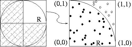

Consider a random point (x,y) in the quadrant. Note the probability it is below the curve is simply the area of the region under the curve compared to the total area of the quadrant. This is simply Pi/4.

To compute Pi using this method, one needs to generate N random points (x,y) in the quadrant. Count the number of these points that are below the curve (x² + y² < R²), a "hit", call this number S. Pi/4 can be approximated as the number of hits divided by the total number of points generated by noting that S/N approaches Pi/4 as N goes to infinity. So 4S/N will be an approxiamte value for Pi. In the above figure N=40 and S=31, so Pi would be computed as 4·31/40 = 3.1.

Task

Write a MIPS program that computes Pi using the Monte Carlo method described above. Generate a random x value, a random y value, then determine if the corresponding point falls under the curve. If so, increment the number of hits. Use the largest N you can, say 1000000 (you might want to start with something like 40).

Deliverables

Send me an email with the MIPS file containing your program. Comment each line and code segment explaining its function.

References

1. Appendix B
2. Knuth, D., The Art of Computer Programming, Vol. 2, 2nd ed., Addison-Wesley, Reading, (1981).
3. Pi Poster
4. Pi Formulas from MathWorld--A Wolfram Web Resource.